Mask-RCNN

Overview of Mask R-CNN usage

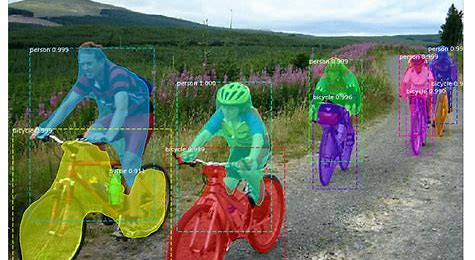
• Mask R-CNN is a powerful model developed by He et al. in 2017. It is currently one of the top models excelling in Instance Segmentation task.
• This model is not only able to pinpoint the location of objects within an image but also to precisely outline the shape of each object.

RoIAlign

RoIAlign Output for a Single RoI

• For a single RoI proposal, after RoIAlign, you get a \(7 \times 7 \times C\) tensor (7x7 bins across C channels).

  Flattening and Feeding into Fully Connected Layers (FCs)

• The \(7 \times 7 \times C\) tensor is flattened into a 1D vector (\(7 \times 7 \times C = 49C\)) before being fed into the fully connected (FC) layers.
• Each RoI produces one flattened vector.

  For Multiple RoIs

• If there are \(N\) RoI proposals for one image, RoIAlign produces \(N\) feature tensors:
  \(N \times 7 \times 7 \times C\)
• These tensors are flattened into \(N\) vectors of size \(49C\), resulting in a tensor of shape:
  \(N \times 49C\)
• This tensor is then fed into the FC layers.

  For Multiple Images (Batch)

• If batch size = 2 (2 images), and each image has \(N_1\) and \(N_2\) RoI proposals, the total output from RoIAlign is:
  \((N_1 + N_2) \times 7 \times 7 \times C\)
• After flattening, it becomes a \((N_1 + N_2) \times 49C\) tensor, which is fed into the FC layers at once.

Mask Prediction Head

• The input to the Mask Head is the feature map generated by RoIAlign, which performs resizing of RPN proposals to match the feature map provided by the backbone. RoIAlign uses bilinear interpolation to map the proposals to a fixed spatial size (e.g., \(14 × 14\)), preserving spatial details. This fixed-size feature map is then fed into the Mask Head for further processing.

1. Classification and Bounding Box Regression Branches

These branches correspond to the Faster R-CNN head (the upper portion of the diagram).

---

Inputs:

• RoI feature map of size \(7 \times 7 \times 256\), generated by RoIAlign.

---

Architecture:

1. Two Fully Connected (FC) Layers:
   • Input: The \(7 \times 7 \times 256\) feature map is flattened into a 1D tensor.
   • Two dense layers with 1024 units each are applied in sequence.
   • Activation: ReLU after each dense layer.
2. Parallel Outputs:
   • Classification Head:
     • A softmax layer produces class probabilities for all \(C\) classes (including the background class).
   • Bounding Box Regression Head:
     • A separate linear layer predicts 4 bounding box offsets for each of the \(C\) classes.
       (4 values per box: \((\Delta x, \Delta y, \Delta w, \Delta h)\)).

---

Output:

• Class scores: \(N \times C\) (for \(C\) classes).
• Bounding box offsets: \(N \times 4C\) (for \(C\) classes, each having 4 regression values).

---

2. Mask Prediction Branch

This branch focuses on per-pixel instance mask prediction (the lower part of the diagram).

---

Inputs:

• RoI feature map of size \(14 \times 14 \times 256\), generated by RoIAlign.
  (Note: This branch uses higher-dimensional spatial feature maps than classification/regression to preserve finer spatial details.)

---

Architecture:

1. 4 Convolutional Layers:
   • Feature refinement is performed using 4 sequential convolutional layers.
   • Each layer uses:
     • \(3 \times 3\) kernels,
     • \(256\) filters,
     • Stride = \(1\) (preserving \(14 \times 14\) resolution at every layer).
   • The output remains:

\[14 \times 14 \times 256\]

1. Upsampling via Transposed Convolution (Deconvolution):
   • After the convolutions, a deconvolution (transpose convolution) layer upsamples the feature map from \(14 \times 14\) to \(28 \times 28\).
   • Output size:

\[28 \times 28 \times 256\]

1. Per-Class Binary Mask Prediction:
   • A \(1 \times 1\) convolution reduces the channel depth from \(256\) to \(C\) (one mask per class).
   • For \(C\) classes, this produces \(C\) binary masks, each of resolution \(28 \times 28\).
   • Output shape:

\[28 \times 28 \times C\]

---

Output:

• Predicted binary masks of size \(28 \times 28\), for each class (\(C\)).

---

Summary Table of the Branches

Branch	Input Size	Operations	Output
Classification	\(7 \times 7 \times 256\)	Flatten → 2 Fully Connected Layers (1024 units each) → Softmax	\(N \times C\) (class probs)
Regression	\(7 \times 7 \times 256\)	Flatten → 2 Fully Connected Layers (1024 units each) → Linear	\(N \times 4C\) (bbox offsets)
Mask Prediction	\(14 \times 14 \times 256\)	4 Conv Layers (\(3 \times 3\)) → Transpose Conv (upsample to \(28 \times 28\)) → \(1 \times 1\) Conv (class masks)	\(N \times 28 \times 28 \times C\) (masks)

Resizing Masks Back to Original Scale

After generating the binary masks for each detected object, the masks must be resized and mapped to their corresponding locations in the original image:

Steps:

1. Map Predicted Mask to Object’s Bounding Box:
   • Each predicted binary mask has a fixed resolution of \(28 \times 28\).
   • The mask is resized to match the dimensions of the object’s bounding box in the original image, denoted as \(W \times H\).
   • The resizing process is typically done using bilinear interpolation, ensuring smoothness and spatial accuracy.

\[\text{Predicted Mask: } 28 \times 28 \xrightarrow{\text{Resize}} W \times H \text{ (Bounding Box Dimensions)}\]

1. Place the Resized Mask in the Image:
   • Once the mask is resized, it is projected back onto the original image by placing it within the corresponding bounding box.
   • Pixels outside the bounding box are set to zero (background) or ignored.

\[\text{Resized Mask: } W \times H \xrightarrow{\text{Project}} \text{Place in Original Image Canvas}\]

1. Combine All Masks:
   • After processing all Regions of Interest (RoIs), the resized masks are combined to create a full mask for the entire image.
   • Overlapping areas are resolved using techniques such as taking the mask of the class with the highest probability at a given pixel.

Final Output:

• A full-resolution mask with the same dimensions as the original image is generated.

\(\text{Image Dimensions: } H_{\text{img}} \times W_{\text{img}}\)

• Every pixel at this stage is assigned to one of the detected masks or left as background.

How is Loss Calculated for One Batch?

The overall loss for Mask R-CNN is a combination of several components, and it’s computed for the entire batch or for one image if that’s the batch size.

---

Loss Components

For each image, the following losses are computed over all RoIs:

---

1. Classification Loss ($L_{\text{cls}}$):

• The classification branch produces a softmax output for \(C\) classes (including the background).
• Cross-entropy loss is used for the predicted class probabilities.
• This loss is calculated only for the positive RoIs (those containing objects).

\[L_{\text{cls}} = \frac{1}{N_{\text{cls}}} \sum_{i} \text{CrossEntropy}(p_i, t_i)\]

• \(p_i\): Predicted probability distribution for RoI \(i\).
• \(t_i\): Ground-truth class label for RoI \(i\).
• \(N_{\text{cls}}\): Total number of positive RoIs in the batch.

---

2. Bounding Box Regression Loss ($L_{\text{bbox}}$):

• This is a smooth L1 loss, applied only to the positive RoIs (those assigned to a specific ground-truth object).
• The predicted bounding box offsets \((\Delta x, \Delta y, \Delta w, \Delta h)\) are compared to the ground-truth bounding box offsets.

\[L_{\text{bbox}} = \frac{1}{N_{\text{bbox}}} \sum_{i} \text{SmoothL1}(\hat{t}_i - t_i)\]

• \(\hat{t}_i\): Predicted bounding box offsets for RoI \(i\).
• \(t_i\): Ground-truth bounding box offsets for RoI \(i\).
• \(N_{\text{bbox}}\): Number of positive RoIs.

---

3. Mask Loss ($L_{\text{mask}}$):

• The mask branch predicts binary masks for each class. The mask loss \(L_{\text{mask}}\) is calculated for one predicted mask per RoI, corresponding to the ground-truth class of the object in that RoI.
• Uses binary cross-entropy loss at a pixel level between the predicted mask and the ground-truth mask.

\[L_{\text{mask}} = \frac{1}{N_{\text{mask}}} \sum_{i} \text{BCE}(M_i, G_i)\]

• \(M_i\): Predicted binary mask for RoI \(i\), resized to the mask resolution of \(28 \times 28\).
• \(G_i\): Ground-truth binary mask for RoI \(i\), resized to \(28 \times 28\).
• \(N_{\text{mask}}\): Number of positive RoIs.

---

4. RPN Loss:

The Region Proposal Network (RPN) is responsible for generating region proposals (anchors) for object detection. The RPN loss consists of two components:

1. RPN Classification Loss ($L_{\text{RPN-class}}$):
   • This loss measures how well the RPN predicts whether an anchor is foreground (object) or background (no object).
   • Binary cross-entropy loss is used for the predicted objectness scores.

\[L_{\text{RPN-class}} = \frac{1}{N_{\text{anchors}}} \sum_{i} \text{BCE}(p_i, t_i)\]

• \(p_i\): Predicted objectness score for anchor \(i\).
• \(t_i\): Ground-truth label for anchor \(i\) (1 for object, 0 for background).
• \(N_{\text{anchors}}\): Total number of anchors used in the batch.

1. RPN Regression Loss ($L_{\text{RPN-bbox}}$):
   • This loss measures how well the RPN predicts the bounding box offsets for positive anchors (anchors assigned to ground-truth objects).
   • Smooth L1 loss is used for the bounding box regression.

\[L_{\text{RPN-bbox}} = \frac{1}{N_{\text{positive anchors}}} \sum_{i} \text{SmoothL1}(\hat{t}_i - t_i)\]

• \(\hat{t}_i\): Predicted bounding box offsets for anchor \(i\).
• \(t_i\): Ground-truth bounding box offsets for anchor \(i\).
• \(N_{\text{positive anchors}}\): Number of positive anchors.

---

Total Loss Per Image

The total loss for one image is the sum of all components:

\[L = L_{\text{cls}} + L_{\text{bbox}} + L_{\text{mask}} + L_{\text{RPN-class}} + L_{\text{RPN-bbox}}\]

If multiple images are in a batch, the losses are summed or averaged across the batch.

---

If Masks Are Projected Back: Does the Loss Use the Combined Mask?

No, the loss is not calculated using the combined mask. During training:

1. Individual RoIs are processed independently.
   • For each RoI:
     • The mask loss is calculated by comparing the predicted \(28 \times 28\) binary mask with the corresponding resized \(28 \times 28\) ground-truth mask.
     • This loss calculation is per RoI, not for a combined full image mask.
2. After processing all RoIs for the image, the total mask loss is averaged over all RoIs for the current image.

---

Inference vs. Training

• During inference:
  • The masks are projected back to the original image and combined into a single output.
• During training:
  • The RoIs are not combined into a full-size image for loss calculation. Instead, the predicted and ground-truth masks are compared and evaluated per RoI.